AI对数据进行滚动统计
编辑
0
2025-06-26

提示词
现在有一个DataFrame,日期为index,其中一列是成交价。我需要先将其重新采样,变成以月度为单位,每个月度中存储该月成交价均值的DataFrame。然后在这个新的DataFrame中添加两个列,分别是12个月的滚动均值和滚动标准差,请给出示例代码。
答案
import pandas as pd
import numpy as np

# 1. 创建示例数据(假设df是您的原始DataFrame)
# 假设索引为日期,列'Close'为成交价
# date_range = pd.date_range(start='2020-01-01', end='2023-12-31', freq='D')
# data = {'Close': np.random.rand(len(date_range)) * 100 + 100}  # 模拟价格数据
# df = pd.DataFrame(data, index=date_range)

df = df[['成交价']]

# 2. 月度重采样:计算每月成交价均值
monthly_df = df.resample('M').mean()  # 'M'表示月末频率[2,4](@ref)
monthly_df.rename(columns={'成交价': 'Monthly_Avg'}, inplace=True)

# 3. 计算12个月滚动均值和标准差
monthly_df['Rolling_Mean_12M'] = monthly_df['Monthly_Avg'].rolling(
    window=12,         # 12个月窗口
    min_periods=1      # 至少有1个月数据即可计算
).mean()

monthly_df['Rolling_Std_12M'] = monthly_df['Monthly_Avg'].rolling(
    window=12,
    min_periods=1
).std()

# 查看结果
print(monthly_df.head())
print(monthly_df.tail())
我增加了自己的数据和修改了表格列名的代码,其余都是ai写的。
结果:
            Monthly_Avg  Rolling_Mean_12M  Rolling_Std_12M
日期
2014-01-31    52.351613         52.351613              NaN
2014-02-28    51.359643         51.855628         0.701429
2014-03-31    55.106667         52.939307         1.941414
2014-04-30    54.822333         53.410064         1.843684
2014-05-31    53.120323         53.352116         1.601926
            Monthly_Avg  Rolling_Mean_12M  Rolling_Std_12M
日期
2020-08-31    93.975714         84.484803         6.335345
2020-09-30    86.711819         84.505330         6.342740
2020-10-31    93.042000         85.201932         6.806107
2020-11-30    86.094763         86.330226         5.519682
2020-12-31    78.629130         86.758297         4.547034
使用“加法模型”进行季节性分解
简化代码后加描述。
提示词
# Python代码
# 以月度重新采样为均值
df = df[['成交价']]
monthly_df = df.resample('M').mean()
# 计算12个月的滚动均值和滚动标准差
monthly_df['Rolling_Mean'] = monthly_df['成交价'].rolling(window=12).mean()
monthly_df['Rolling_Std'] = monthly_df['成交价'].rolling(window=12).std()
# 输出包含滚动均值和滚动标准差的dataframe最新5条
monthly_df.tail()
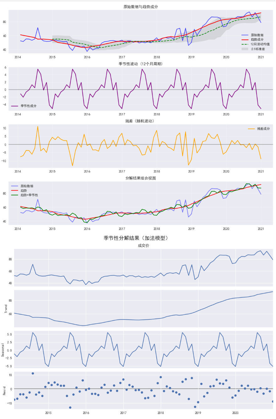
还是上面的monthly_df,我希望使用additive model对其进行季节分解,并将结果进行可视化,请给出示例代码。
答案
import pandas as pd
import matplotlib.pyplot as plt
from statsmodels.tsa.seasonal import seasonal_decompose

# 假设monthly_df是已有的月度数据DataFrame
# 包含'成交价'列以及计算好的滚动均值和滚动标准差
# monthly_df = ... (已有数据)

# 进行季节性分解(加法模型)
result = seasonal_decompose(monthly_df['成交价'],
                           model='additive',
                           period=12,  # 月度数据的周期为12个月
                           extrapolate_trend='freq')  # 避免趋势成分的NaN值[3,7](@ref)

# 提取分解结果
trend = result.trend
seasonal = result.seasonal
residual = result.resid

# 创建可视化图表
plt.figure(figsize=(12, 10))

# 原始数据和趋势项[5](@ref)
plt.subplot(4, 1, 1)
plt.plot(monthly_df.index, monthly_df['成交价'], label='原始数据', color='blue', alpha=0.7)
plt.plot(trend.index, trend, label='趋势成分', color='red', linewidth=2)
plt.plot(monthly_df.index, monthly_df['Rolling_Mean'], label='12月滚动均值',
         color='green', linestyle='--')
plt.fill_between(monthly_df.index,
                 monthly_df['Rolling_Mean'] - monthly_df['Rolling_Std'],
                 monthly_df['Rolling_Mean'] + monthly_df['Rolling_Std'],
                 color='gray', alpha=0.2, label='±1标准差')
plt.title('原始数据与趋势成分')
plt.legend(loc='best')
plt.grid(alpha=0.3)

# 季节性成分[1,3](@ref)
plt.subplot(4, 1, 2)
plt.plot(seasonal.index, seasonal, label='季节性成分', color='purple')
plt.title('季节性波动 (12个月周期)')
plt.axhline(y=0, color='black', linestyle='-', alpha=0.3)
plt.legend(loc='best')
plt.grid(alpha=0.3)

# 残差成分[6](@ref)
plt.subplot(4, 1, 3)
plt.plot(residual.index, residual, label='残差成分', color='orange')
plt.title('残差(随机波动)')
plt.axhline(y=0, color='black', linestyle='-', alpha=0.3)
plt.legend(loc='best')
plt.grid(alpha=0.3)

# 组合视图[5,7](@ref)
plt.subplot(4, 1, 4)
plt.plot(monthly_df.index, monthly_df['成交价'], label='原始数据', color='blue', alpha=0.5)
plt.plot(trend.index, trend, label='趋势', color='red')
plt.plot(trend.index, trend + seasonal, label='趋势+季节性', color='green')
plt.title('分解结果组合视图')
plt.legend(loc='best')
plt.grid(alpha=0.3)

plt.tight_layout()
plt.show()

# 可选:单独绘制statsmodels自带的分解图[3](@ref)
fig = result.plot()
fig.set_size_inches(12, 8)
fig.suptitle('季节性分解结果(加法模型)', fontsize=16)
plt.tight_layout()
plt.show()
图像:
使用STL分解法进行时间序列分解
简化代码后加描述。
提示词
# Python代码
# 以月度重新采样为均值
df = df[['成交价']]
monthly_df = df.resample('M').mean()
# 计算12个月的滚动均值和滚动标准差
monthly_df['Rolling_Mean'] = monthly_df['成交价'].rolling(window=12).mean()
monthly_df['Rolling_Std'] = monthly_df['成交价'].rolling(window=12).std()
# 输出包含滚动均值和滚动标准差的dataframe最新5条
monthly_df.tail()
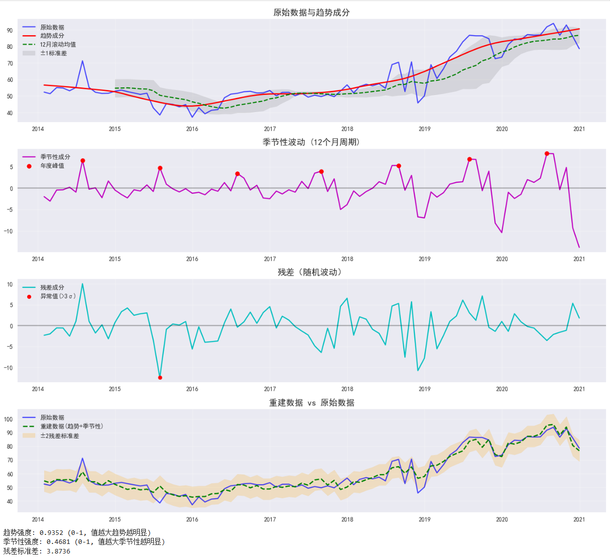
继续使用monthly_df这个DataFrame,用STL分解法对其进行季节性分解,并将结果进行可视化,请给出示例代码。
答案
import pandas as pd
import numpy as np
import matplotlib.pyplot as plt
from statsmodels.tsa.seasonal import STL

# 确保数据没有缺失值(STL要求完整数据)
monthly_df = monthly_df.dropna(subset=['成交价'])

# 执行STL分解(加法模型)
stl = STL(monthly_df['成交价'], period=12)  # 月度数据周期为12个月
result = stl.fit()

# 提取分解结果
trend = result.trend
seasonal = result.seasonal
residual = result.resid

# 创建专业级可视化图表
plt.figure(figsize=(14, 12))

# 1. 原始数据与趋势成分
plt.subplot(4, 1, 1)
plt.plot(monthly_df.index, monthly_df['成交价'], 'b-', label='原始数据', alpha=0.7)
plt.plot(trend.index, trend, 'r-', linewidth=2, label='趋势成分')
plt.plot(monthly_df.index, monthly_df['Rolling_Mean'], 'g--', label='12月滚动均值')
plt.fill_between(monthly_df.index,
                 monthly_df['Rolling_Mean'] - monthly_df['Rolling_Std'],
                 monthly_df['Rolling_Mean'] + monthly_df['Rolling_Std'],
                 color='gray', alpha=0.2, label='±1标准差')
plt.title('原始数据与趋势成分', fontsize=14)
plt.legend(loc='upper left')
plt.grid(alpha=0.3)

# 2. 季节性成分
plt.subplot(4, 1, 2)
plt.plot(seasonal.index, seasonal, 'm-', label='季节性成分')
# 标记季节性峰值
peak_idx = seasonal.groupby(seasonal.index.year).idxmax()
plt.scatter(peak_idx, seasonal.loc[peak_idx], color='red', s=50, zorder=5, label='年度峰值')
plt.axhline(y=0, color='k', linestyle='-', alpha=0.3)
plt.title('季节性波动 (12个月周期)', fontsize=14)
plt.legend(loc='upper left')
plt.grid(alpha=0.3)

# 3. 残差成分
plt.subplot(4, 1, 3)
plt.plot(residual.index, residual, 'c-', label='残差成分')
plt.axhline(y=0, color='k', linestyle='-', alpha=0.3)
# 标记异常残差(超过3个标准差)
std_resid = residual.std()
outliers = residual[np.abs(residual) > 3 * std_resid]
plt.scatter(outliers.index, outliers, color='red', s=40, zorder=5, label='异常值(>3σ)')
plt.title('残差(随机波动)', fontsize=14)
plt.legend(loc='upper left')
plt.grid(alpha=0.3)

# 4. 重建数据与原始数据对比
plt.subplot(4, 1, 4)
reconstructed = trend + seasonal  # 趋势 + 季节性
plt.plot(monthly_df.index, monthly_df['成交价'], 'b-', label='原始数据', alpha=0.7)
plt.plot(reconstructed.index, reconstructed, 'g--', linewidth=2, label='重建数据(趋势+季节性)')
plt.fill_between(residual.index,
                 reconstructed - 2 * std_resid,
                 reconstructed + 2 * std_resid,
                 color='orange', alpha=0.2, label='±2残差标准差')
plt.title('重建数据 vs 原始数据', fontsize=14)
plt.legend(loc='upper left')
plt.grid(alpha=0.3)

plt.tight_layout()
plt.show()

# 计算并显示分解指标
trend_strength = max(0, 1 - residual.var() / (monthly_df['成交价'] - seasonal).var())
seasonal_strength = max(0, 1 - residual.var() / (monthly_df['成交价'] - trend).var())

print(f"趋势强度: {trend_strength:.4f} (0-1, 值越大趋势越明显)")
print(f"季节性强度: {seasonal_strength:.4f} (0-1, 值越大季节性越明显)")
print(f"残差标准差: {residual.std():.4f}")
图像:
- 0
- 0
-
赞助
 支付宝
支付宝
 微信
微信
-
分享