提示词

以日期为index的DataFrame，频率为月度，包含一列商品的成交价，现在需要使用Python调用指数平滑方法对其进行建模，首先要将数据拆分成训练集和测试机，用训练集拟合模型，再对测试集进行预测，并将结果可视化，请给出示例代码。

答案

import pandas as pd
import numpy as np
import matplotlib.pyplot as plt
from statsmodels.tsa.holtwinters import ExponentialSmoothing
from sklearn.metrics import mean_squared_error, mean_absolute_error
from sklearn.model_selection import TimeSeriesSplit

# 1. 准备示例数据（替换为实际数据）
# dates = pd.date_range(start='2018-01-01', end='2025-06-01', freq='M')
# prices = np.cumsum(np.random.normal(0.5, 2, len(dates))) + 100  # 模拟成交价
# df = pd.DataFrame({'成交价': prices}, index=dates)
# print("原始数据示例:")
# print(df.head())

# 2. 数据拆分 - 按时间顺序划分训练集和测试集[8](@ref)
train_size = int(len(monthly_df) * 0.8)  # 80%作为训练集
train = monthly_df.iloc[:train_size]
test = monthly_df.iloc[train_size:]

print(f"\n训练集: {train.index.min()} 至 {train.index.max()} ({len(train)}个月)")
print(f"测试集: {test.index.min()} 至 {test.index.max()} ({len(test)}个月)")

# 3. 模型拟合 - 使用Holt-Winters季节性指数平滑[2,6](@ref)
model = ExponentialSmoothing(
    train['成交价'],
    trend='add',               # 加法趋势
    seasonal='add',            # 加法季节性
    seasonal_periods=12,       # 月度数据的年度季节性周期
    damped_trend=True          # 使用阻尼趋势防止预测发散[1](@ref)
).fit()

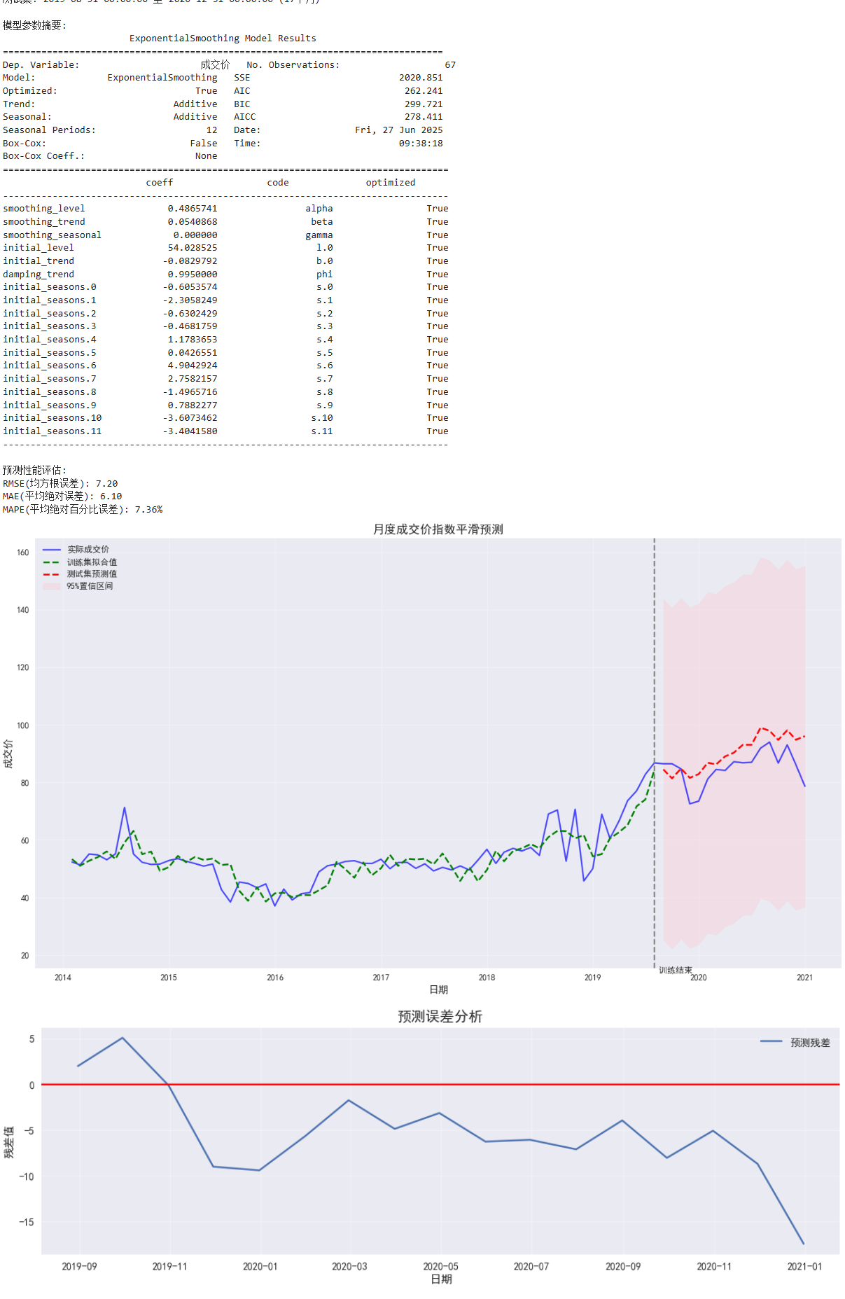
print("\n模型参数摘要:")
print(model.summary())

# 4. 预测测试集
forecast = model.forecast(steps=len(test))
forecast_df = pd.DataFrame(forecast, index=test.index, columns=['预测值'])

# 5. 评估预测性能
rmse = np.sqrt(mean_squared_error(test['成交价'], forecast))
mae = mean_absolute_error(test['成交价'], forecast)
mape = np.mean(np.abs((test['成交价'] - forecast) / test['成交价'])) * 100

print("\n预测性能评估:")
print(f"RMSE(均方根误差): {rmse:.2f}")
print(f"MAE(平均绝对误差): {mae:.2f}")
print(f"MAPE(平均绝对百分比误差): {mape:.2f}%")

# 6. 可视化结果
plt.figure(figsize=(14, 8))

# 绘制原始数据和拟合值
plt.plot(monthly_df.index, monthly_df['成交价'], 'b-', label='实际成交价', alpha=0.7)
plt.plot(train.index, model.fittedvalues, 'g--', label='训练集拟合值', linewidth=2)

# 绘制预测值和置信区间
plt.plot(forecast_df.index, forecast_df['预测值'], 'r--', label='测试集预测值', linewidth=2)
plt.fill_between(
    forecast_df.index,
    model.forecast(steps=len(test)) - 1.96 * model.sse / len(train),
    model.forecast(steps=len(test)) + 1.96 * model.sse / len(train),
    color='pink', alpha=0.3, label='95%置信区间'
)

# 添加分隔线和标注
plt.axvline(x=train.index[-1], color='gray', linestyle='--')
plt.text(train.index[-1], plt.ylim()[0]*0.9, ' 训练结束', fontsize=10)

# 图表装饰
plt.title('月度成交价指数平滑预测', fontsize=14)
plt.xlabel('日期', fontsize=12)
plt.ylabel('成交价', fontsize=12)
plt.grid(alpha=0.3)
plt.legend(loc='upper left')
plt.tight_layout()

# 7. 残差诊断（可选）
residuals = test['成交价'] - forecast
plt.figure(figsize=(14, 4))
plt.plot(residuals, label='预测残差')
plt.axhline(y=0, color='r', linestyle='-')
plt.title('预测误差分析', fontsize=14)
plt.xlabel('日期')
plt.ylabel('残差值')
plt.grid(alpha=0.3)
plt.legend()
plt.show()

代码都是ai写的。

结果：