提示词

现有一个名为returns的DataFrame，其中包含一个投资组合中两只股票的每日简单收益，两只股票的权重相同，现在需要演示VaR的估计，并且最后用直方图可视化VaR估计结果，请给出示例代码。

答案

import numpy as np
import pandas as pd
import matplotlib.pyplot as plt
from scipy.stats import genpareto

# 假设returns是包含两列股票收益的DataFrame（列名：stock1, stock2）
# 生成示例数据（实际使用时替换为您的returns）
# np.random.seed(42)
# dates = pd.date_range(start="2024-01-01", periods=500)
# returns = pd.DataFrame({
#     'stock1': np.random.normal(0.001, 0.02, 500),
#     'stock2': np.random.normal(0.0005, 0.015, 500)
# }, index=dates)

# ===== 1. 计算投资组合收益（等权重）=====
weights = np.array([0.5, 0.5])  # 等权重
portfolio_returns = returns.dot(weights)  # 组合每日收益

# ===== 2. 计算历史模拟法VaR（95%置信度）=====
confidence_level = 0.95
sorted_returns = np.sort(portfolio_returns)  # 收益从小到大排序
var_index = int(len(sorted_returns) * (1 - confidence_level))
var_value = -sorted_returns[var_index]  # VaR取正值（损失金额）

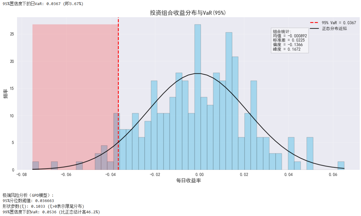
print(f"95%置信度下的日VaR: {var_value:.4f} (即{var_value*100:.2f}%)")

# ===== 3. 直方图可视化VaR结果 =====
plt.figure(figsize=(12, 6))

# 绘制收益分布直方图
n, bins, patches = plt.hist(
    portfolio_returns,
    bins=50,
    alpha=0.7,
    color='skyblue',
    edgecolor='black',
    density=True
)

# 标注VaR线
plt.axvline(x=-var_value, color='red', linestyle='--', linewidth=2, 
            label=f'95% VaR = {var_value:.4f}')
plt.fill_betweenx([0, max(n)], -var_value, sorted_returns.min(), 
                 color='red', alpha=0.2)

# 添加分布曲线
plt.plot(bins, 
         norm.pdf(bins, portfolio_returns.mean(), portfolio_returns.std()), 
         'k-', linewidth=1.5, label='正态分布近似')

# 美化图表
plt.title('投资组合收益分布与VaR(95%)', fontsize=14)
plt.xlabel('每日收益率', fontsize=12)
plt.ylabel('频率', fontsize=12)
plt.legend()
plt.grid(alpha=0.3)

# 添加统计信息框
stats_text = (
    f"组合统计:\n"
    f"均值 = {portfolio_returns.mean():.6f}\n"
    f"标准差 = {portfolio_returns.std():.4f}\n"
    f"偏度 = {pd.Series(portfolio_returns).skew():.4f}\n"
    f"峰度 = {pd.Series(portfolio_returns).kurtosis():.4f}"
)
plt.gcf().text(0.75, 0.75, stats_text, bbox=dict(facecolor='white', alpha=0.5), 
              fontsize=10)

plt.tight_layout()
plt.savefig('VaR_visualization.png', dpi=300)
plt.show()

# ===== 4. 极端风险分析（广义帕累托分布）=====
# 计算损失数据（取负收益）
losses = -portfolio_returns
threshold = np.percentile(losses, 95)  # 95%分位数作为阈值
exceedances = losses[losses > threshold] - threshold  # 超阈值损失

# 拟合广义帕累托分布（GPD）
shape, loc, scale = genpareto.fit(exceedances, floc=0)

# 计算99%置信度下的VaR
alpha = 0.99
n_obs = len(losses)
n_exceed = len(exceedances)
var_gpd = threshold + (scale / shape) * (((1 - alpha) * n_obs / n_exceed) ** (-shape) - 1)

print(f"\n极端风险分析（GPD模型）:")
print(f"95%分位数阈值: {threshold:.6f}")
print(f"形状参数(ξ): {shape:.4f} (ξ>0表示厚尾分布)")
print(f"99%置信度下的VaR: {var_gpd:.4f} (比正态估计高{100*(var_gpd/var_value-1):.1f}%)")

结果：