提示词

# Python代码
# 以月度重新采样为均值
df = df[['成交价']]
monthly_df = df.resample('M').mean()

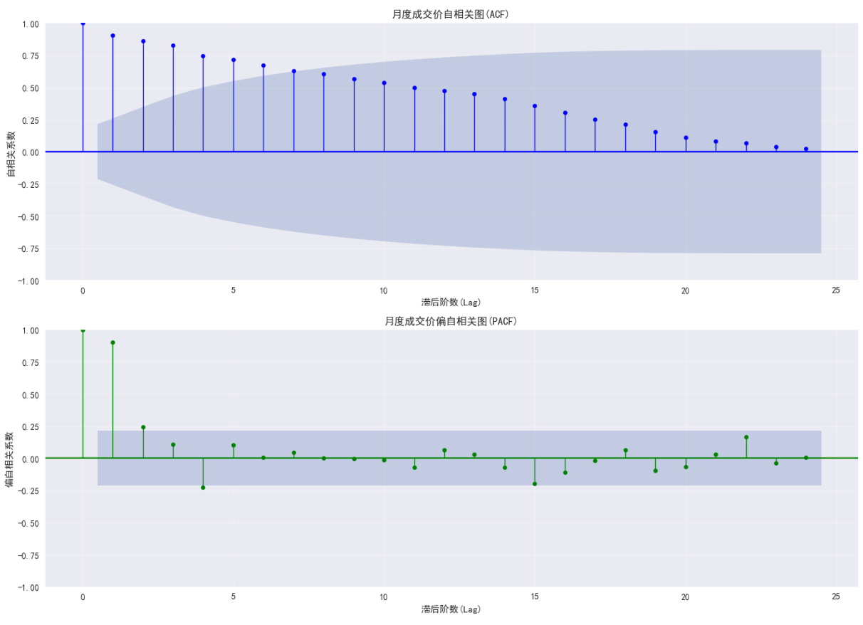
在monthly_df中，有一列成交价，需要绘制该字段的自相关图和偏自相关图，请给出示例代码。

答案

import matplotlib.pyplot as plt
from statsmodels.graphics.tsaplots import plot_acf, plot_pacf

# 确保数据没有缺失值
monthly_df = monthly_df.dropna(subset=['成交价'])

# 设置图形大小
plt.figure(figsize=(14, 10))

# 绘制自相关图(ACF)
plt.subplot(2, 1, 1)
plot_acf(monthly_df['成交价'], lags=24, ax=plt.gca(), 
         title='月度成交价自相关图(ACF)', color='blue', 
         vlines_kwargs={'colors':'blue', 'linewidth':1})
plt.grid(alpha=0.3)
plt.xlabel('滞后阶数(Lag)')
plt.ylabel('自相关系数')

# 绘制偏自相关图(PACF)
plt.subplot(2, 1, 2)
plot_pacf(monthly_df['成交价'], lags=24, ax=plt.gca(), 
          title='月度成交价偏自相关图(PACF)', color='green',
          vlines_kwargs={'colors':'green', 'linewidth':1})
plt.grid(alpha=0.3)
plt.xlabel('滞后阶数(Lag)')
plt.ylabel('偏自相关系数')

# 调整布局并显示
plt.tight_layout()
plt.show()

代码都是ai写的。

结果：

确定模型阶数pdq

提示词

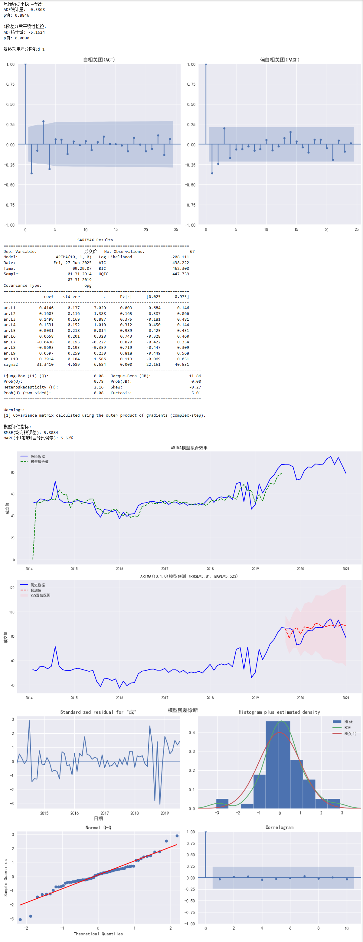
以日期为index的DataFrame，包含某产品的成交价，需要对这列数据用ARIMA建模，并对模型进行评估，最后将原始数据和模型预测结果进行可视化，请给出示例代码。

答案

import pandas as pd
import numpy as np
import matplotlib.pyplot as plt
from statsmodels.tsa.stattools import adfuller
from statsmodels.graphics.tsaplots import plot_acf, plot_pacf
from statsmodels.tsa.arima.model import ARIMA
from sklearn.metrics import mean_squared_error
import warnings

# 忽略警告信息
warnings.filterwarnings('ignore')

# 1. 数据准备（假设df是包含日期索引和'成交价'列的DataFrame）
# 确保索引是DatetimeIndex格式
# df.index = pd.to_datetime(df.index)

# 2. 平稳性检验与差分处理
def check_stationarity(series):
    """执行ADF检验并返回结果"""
    result = adfuller(series.dropna())
    print(f'ADF统计量: {result[0]:.4f}')
    print(f'p值: {result[1]:.4f}')
    return result[1] < 0.05  # p<0.05表示平稳

# 检查原始数据平稳性
print("原始数据平稳性检验:")
is_stationary = check_stationarity(monthly_df['成交价'])

# 自动差分直到平稳
d = 0
diff_series = monthly_df['成交价'].copy()
while not is_stationary and d < 3:  # 最多差分3次
    d += 1
    diff_series = diff_series.diff().dropna()
    print(f"\n{d}阶差分后平稳性检验:")
    is_stationary = check_stationarity(diff_series)

print(f"\n最终采用差分阶数d={d}")

# 3. 确定ARIMA参数(p,d,q)
# 绘制ACF和PACF图
plt.figure(figsize=(12, 6))
plt.subplot(121)
plot_acf(diff_series, lags=24, ax=plt.gca(), title='自相关图(ACF)')
plt.subplot(122)
plot_pacf(diff_series, lags=24, ax=plt.gca(), title='偏自相关图(PACF)')
plt.tight_layout()
plt.show()

# 4. 划分训练集和测试集
train_size = int(len(monthly_df) * 0.8)  # 80%作为训练集
train = monthly_df.iloc[:train_size]
test = monthly_df.iloc[train_size:]

# 5. 拟合ARIMA模型 (参数需根据ACF/PACF调整)
p, q = 10, 0  # 根据ACF/PACF截尾情况确定 按示例10，1
model = ARIMA(train['成交价'], order=(p, d, q))
model_fit = model.fit()
print(model_fit.summary())

# 6. 模型评估
# 在测试集上进行预测
forecast = model_fit.get_forecast(steps=len(test))
forecast_mean = forecast.predicted_mean
conf_int = forecast.conf_int()

# 计算评估指标
rmse = np.sqrt(mean_squared_error(test['成交价'], forecast_mean))
mape = np.mean(np.abs((test['成交价'] - forecast_mean) / test['成交价'])) * 100

print(f'\n模型评估指标:')
print(f'RMSE(均方根误差): {rmse:.4f}')
print(f'MAPE(平均绝对百分比误差): {mape:.2f}%')

# 7. 可视化结果
plt.figure(figsize=(14, 10))

# 原始数据与拟合值
plt.subplot(2, 1, 1)
plt.plot(monthly_df.index, monthly_df['成交价'], 'b-', label='原始数据')
plt.plot(train.index, model_fit.fittedvalues, 'g--', label='模型拟合值')
plt.title('ARIMA模型拟合效果')
plt.ylabel('成交价')
plt.legend()
plt.grid(alpha=0.3)

# 预测结果与置信区间
plt.subplot(2, 1, 2)
plt.plot(monthly_df.index, monthly_df['成交价'], 'b-', label='历史数据')
plt.plot(forecast_mean.index, forecast_mean, 'r--', label='预测值')
plt.fill_between(conf_int.index,
                 conf_int.iloc[:, 0],
                 conf_int.iloc[:, 1],
                 color='pink', alpha=0.3, label='95%置信区间')
plt.title(f'ARIMA({p},{d},{q})模型预测 (RMSE={rmse:.2f}, MAPE={mape:.2f}%)')
plt.ylabel('成交价')
plt.legend()
plt.grid(alpha=0.3)

plt.tight_layout()
plt.show()

# 8. 残差诊断（可选）
model_fit.plot_diagnostics(figsize=(12, 8))
plt.suptitle('模型残差诊断', y=0.95)
plt.tight_layout()
plt.show()

结果：